Available Algorithms
This section provides an overview of the available hyperparameter optimization algorithms in Sherpa. Below is a table that discusses use cases for each algorithm. This is followed by a short comparison benchmark and the algorithms themselves.
| Use cases | |
Grid Search
|
Great for understanding the
impact of one or two parameters.
|
Random Search
|
More efficient than grid search when used with many
hyperparameters. Great for getting
a full picture of the impact of many hyperparameters
since hyperparameters are uniformly sampled from the
whole space.
|
GPyOpt Bayesian
Optimization
|
More efficient than Random search when the number of
trials is sufficiently large.
|
Asynchronous
Successive
Halving
|
Due to its early stopping, especially useful when it
would otherwise be infeasible to run a hyperparameter
optimization because of the computational cost.
|
Local Search
|
Can quickly explore “tweaks” to a model that is
already good while using less trials than Random search
or Bayesian optimization.
|
Population
Based
Training
|
Can discover schedules of training parameters and is
therefore especially good for learning rate, momentum,
batch size, etc.
|
For the specification of each algorithm see below.
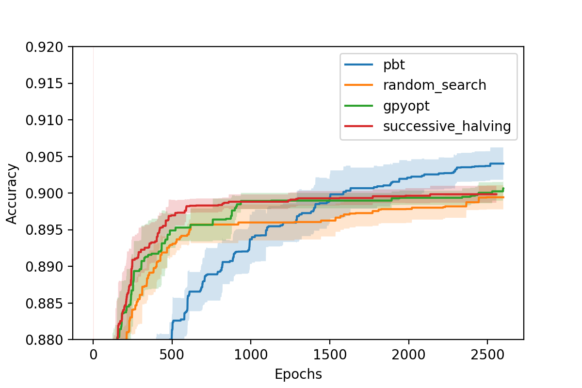
Comparison using Fashion MNIST MLP
We constructed a simple and fast to run benchmark to run these algorithms on. This uses a fully connected neural
network trained on the Fashion MNIST dataset. The tuning parameters are the learning rate, the learning rate
decay, the momentum, minibatch size, and the dropout rate. We compare Random Search, GPyOpt, Population Based Training (pbt),
and Successive Halving. All algorithms are allowed an equal budget corresponding to 100 models trained for 26 epochs. The
plot below shows the mean taken over five runs of each algorithm. The shaded regions correspond to two standard deviations.
On the y-axis is the classification accuracy of the best model found. On the x-axis are the epochs spent. We run 20 evaluations
in parallel. Note that the results of GPyOpt may be impacted by the high number of parallel evaluations. The code to reproduce
this benchmark can be found at sherpa/examples/parallel-examples/fashion_mnist_benchmark.
The currently available algorithms in Sherpa are listed below:
Grid Search
-
class
sherpa.algorithms.GridSearch(num_grid_points=2)[source] Explores a grid across the hyperparameter space such that every pairing is evaluated.
For continuous and discrete parameters grid points are picked within the range. For example, a continuous parameter with range [1, 2] with two grid points would have points 1 1/3 and 1 2/3. For three points, 1 1/4, 1 1/2, and 1 3/4.
Example:
hp_space = {'act': ['tanh', 'relu'],
            'lrinit': [0.1, 0.01],
            }
parameters = sherpa.Parameter.grid(hp_space)
alg = sherpa.algorithms.GridSearch()
Parameters: num_grid_points (int) – number of grid points for continuous / discrete.
Random Search
-
class
sherpa.algorithms.RandomSearch(max_num_trials=None)[source] Random Search with a repeat option.
Trials parameter configurations are uniformly sampled from their parameter ranges. The repeat option allows to re-run a trial repeat number of times. By default this is 1.
Parameters: - max_num_trials (int) – number of trials, otherwise runs indefinitely.
- repeat (int) – number of times to repeat a parameter configuration.
Bayesian Optimization with GPyOpt
-
class
sherpa.algorithms.GPyOpt(model_type='GP', num_initial_data_points='infer', initial_data_points=[], acquisition_type='EI', max_concurrent=4, verbosity=False, max_num_trials=None)[source] Sherpa wrapper around the GPyOpt package (https://github.com/SheffieldML/GPyOpt).
Parameters: - model_type (str) – The model used: - ‘GP’, standard Gaussian process. - ‘GP_MCMC’, Gaussian process with prior in the hyper-parameters. - ‘sparseGP’, sparse Gaussian process. - ‘warperdGP’, warped Gaussian process. - ‘InputWarpedGP’, input warped Gaussian process - ‘RF’, random forest (scikit-learn).
- num_initial_data_points (int) – Number of data points to collect before fitting model. Needs to be greater/equal to the number of hyper- parameters that are being optimized. Using default ‘infer’ corres- ponds to number of hyperparameters + 1 or 0 if results are not empty.
- initial_data_points (list[dict] or pandas.Dataframe) – Specifies initial data points. If len(initial_data_points)<num_initial_data_points then the rest is randomly sampled. Use this option to provide hyperparameter configurations that are known to be good.
- acquisition_type (str) – Type of acquisition function to use. - ‘EI’, expected improvement. - ‘EI_MCMC’, integrated expected improvement (requires GP_MCMC model). - ‘MPI’, maximum probability of improvement. - ‘MPI_MCMC’, maximum probability of improvement (requires GP_MCMC model). - ‘LCB’, GP-Lower confidence bound. - ‘LCB_MCMC’, integrated GP-Lower confidence bound (requires GP_MCMC model).
- max_concurrent (int) – The number of concurrent trials. This generates a batch of max_concurrent trials from GPyOpt to evaluate. If a new observation becomes available, the model is re-evaluated and a new batch is created regardless of whether the previous batch was used up. The used method is local penalization.
- verbosity (bool) – Print models and other options during the optimization.
- max_num_trials (int) – maximum number of trials to run for.
Asynchronous Successive Halving aka Hyperband
-
class
sherpa.algorithms.SuccessiveHalving(r=1, R=9, eta=3, s=0, max_finished_configs=50)[source] Asynchronous Successive Halving as described in:
@article{li2018massively, title={Massively parallel hyperparameter tuning}, author={Li, Liam and Jamieson, Kevin and Rostamizadeh, Afshin and Gonina, Ekaterina and Hardt, Moritz and Recht, Benjamin and Talwalkar, Ameet}, journal={arXiv preprint arXiv:1810.05934}, year={2018} }Asynchronous successive halving operates based on the multi-armed bandit algorithm Successive Halving (SHA) and performs principled early stopping for random search.
Parameters: - r (int) – minimum resource that each configuration will be trained for.
- R (int) – maximum resource.
- eta (int) – elimination rate.
- s (int) – minimum early-stopping rate.
- max_finished_configs (int) – stop once max_finished_configs models have been trained to completion.
Local Search
-
class
sherpa.algorithms.LocalSearch(seed_configuration, perturbation_factors=(0.8, 1.2), repeat_trials=1)[source] Local Search Algorithm.
This algorithm expects to start with a very good hyperparameter configuration. It changes one hyperparameter at a time to see if better results can be obtained.
Parameters: - seed_configuration (dict) – hyperparameter configuration to start with.
- perturbation_factors (Union[tuple,list]) – continuous parameters will be multiplied by these.
- repeat_trials (int) – number of times that identical configurations are repeated to test for random fluctuations.
Population Based Training
-
class
sherpa.algorithms.PopulationBasedTraining(num_generations, population_size=20, parameter_range={}, perturbation_factors=(0.8, 1.2))[source] Population based training (PBT) as introduced by Jaderberg et al. 2017.
PBT trains a generation of
population_sizeseed trials (randomly initialized) for a user specified number of iterations e.g. one epoch. The top 80% then move on unchanged into the second generation. The bottom 20% are re-sampled from the top 20% and perturbed. The second generation again trains for the same number of iterations and the same procedure is repeated to move into the third generation etc.Parameters: - num_generations (int) – the number of generations to run for.
- population_size (int) – the number of randomly intialized trials at the beginning and number of concurrent trials after that.
- parameter_range (dict[Union[list,tuple]) – upper and lower bounds beyond which parameters cannot be perturbed.
- perturbation_factors (tuple[float]) – the factors by which continuous parameters are multiplied upon perturbation; one is sampled randomly at a time.
Repeat
-
class
sherpa.algorithms.Repeat(algorithm, num_times=5, wait_for_completion=False, agg=False)[source] Takes another algorithm and repeats every hyperparameter configuration a given number of times. The wrapped algorithm will be passed the mean objective values of the repeated experiments.
Parameters: - algorithm (sherpa.algorithms.Algorithm) – the algorithm to produce hyperparameter configurations.
- num_times (int) – the number of times to repeat each configuration.
- wait_for_completion (bool) – only relevant when running in parallel with max_concurrent > 1. Means that the algorithm won’t issue the next suggestion until all repetitions are completed. This can be useful when the repeats have impact on sequential decision making in the wrapped algorithm.
- agg (bool) – whether to aggregate repetitions before passing them to the parameter generating algorithm.